Skewed Data: Finding The Columns
While in the process of looking for a job that led to the position that I currently hold, I interviewed for a job at a recognizably-named company that was struggling to keep up with their “statistics.” I have a confession. I had no idea what “statistics” were in the SQL Server world. I wasn’t offered that job, but in the interim I did a lot of reading and research on the SQL Server notion of “statistics.” Luckily, I was offered a position at another company a few months later. This company sent me to my very first PASS Summit (2013) in Charlotte, NC where I sat in on Kimberly Tripp’s “Skewed Data, Poor Cardinality Estimates, and Plans Gone Bad” session 1. This session was extremely helpful as it helped me to not only get a demonstration-based idea of how SQL Server actually used Statistics. Naturally, I raced home and tried to apply all that I knew. I looked for skew and I added filtered Statistics all over the place.
Fast-forward two years and I realize that may not have been the best plan of action. Instead of just blindly analyzing histogram windows, I decided that what I needed to do was look at how severely skewed the data might actually be because what I didn’t previously have was a notion of where to start with the analysis. I’d stumbled across Richie Rump’s sp_DataProfile2, which is excellent, but didn’t fit my exact use case. So I set about coming up with a table skew analysis method that would point me in the direction of where I should set up further investigations into skewed Statistics.
The Theory
Creating the Histogram Buckets
At the core of distribution analysis is the notion of the histogram. Essentially a histogram is a diagram of the frequency of values within a given interval. Because I want an accurate representation of the data in the table(s) that I analyze, I choose an interval of 1, which is to say, I want to count the frequency of each value in the column. The code for this process is pretty straightforward.
[code lang=“text”] select [key] = [sentence_id], [x] = dense_rank() over (order by [sentence_id]), [f] = count_big(1) into tempdb.dbo.[tt_f_word_sentence_id] from [dbo].[f_word] tablesample system (59 percent) where [sentence_id] is not null group by [sentence_id] [/code]
A few notes. I rank over the key value because:
it’s how histograms work.
later we’re going to need to find the average. What’s the average of 2014-11-05, 2014-11-06, 2015-09-23, 2016-01-07, or the average of ‘process a’,‘process z’,‘process a’,‘process k’?
I can index on an integer, but not on a
VARCHAR(4000)which may, or may not, exist in a table.
Calculating “Skewness”
Once we’ve generated the histogram, we need to determine if the data is skewed. I knew of skewness calculations (because my wife’s a stats wiz), but Brown University’s page3 made the calculation accessible for me.
[code lang=“text”]
select
…
sk.b1,
sk.G1,
sk.ses,
…,
Zg1 = (100. * d)/n,
…,
(100.d)/574236 — <- table cardinality, zG1 = case sk.ses when 0 then sk.G1 else sk.G1/sk.ses end from ( select b1 = case when (power(m2,1.5)) = 0 then 0 else m3 / (power(m2,1.5)) end, G1 = (sqrt(1.(n*(n-1)))/(n-2)) * case when (power(m2,1.5)) = 0 then 0 else m3 / (power(m2,1.5)) end, ses = case when ((n-2.)(n+1.)(n+3.)) = 0 then 0 else sqrt(((1.*(6.n)(n-1.)))/((n-2.)(n+1.)(n+3.))) end, d,n from ( select n, d, m2 = sum(power((x-(sxf/n)),2)*f)/n, m3 = sum(power((x-(sxf/n)),3)*f)/n from ( select x, f, sxf = 1.*sum(x*f) over(), n = sum(f) over(), d = count(x) over() from tempdb.dbo.[tt_f_word_sentence_id] ) base group by n,d ) agg ) sk As mentioned earlier, the salient calculations are `b1`, `G1`, `ses`, and `Zg1`. These represent Skewness, Bias-Adjusted (Sample) Skewness, Standard Error of Skewness, and the Skewness Test Statistic, respectively. On their own, b1 and G1 would be helpful measures if there was a table of critical values for them at the scale I've been running (n=24 billion). However, I could only find tables that got up to ~n=1,500. This is where the Standard Error number is helpful. It helps us calculate the deviation from normal for the value we've calculated for Skewness. We divide `G1` by `ses` to calculate our Skewness Test Statistic (`Zg1`). According to the aforementioned Brown article, we can roughly say that anything greater than the absolute value of 2 represents a potential for skew. If `Zg1 > 2` then we're probably positively skewed, which would mean values of x greater than the mean are more prevalent in the data set. ### Analysis Well that's cool and all, but how do I use it? This is where we can merge our understanding of SQL Server Statistics with the more broad discipline of Statistics. This query select * from tempdb.dbo.table_analysis where abs(Zg1) >= 2
and distinct_values >= 100 – if it’s highly skewed but has fewer than 100 distinct values, I don’t care
order by abs(Zg1) desc
[/code]
yields this result:
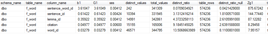
I analyzed the f_word table (word fact table) in my database of greek texts. In this fact table, the sentence_word_id column presented with the greatest value for skewness. This makes sense because sentences have varying numbers of words. Because it is highly positive (Zg1 = 875.67242), we’d conclude that most sentences have more words than the average Greek sentence (in my analyzed corpus). However, the column only has 242 distinct values so the chances that the skew actually matters is pretty small. With so few distinct values, over against a data set of 574,236 rows the density is .04%, which is generally able to be accounted for through histogram compression.4 In fact, using the data in the screenshot above, I’d focus on the word_id column as it has the largest density (distinct_ratio) for non-null values, and presents with Zg1 = 7.95157.
So What?
In the upcoming days (weeks? months? who knows, at the rate I blog) I’ll discuss how to take action on this initial analysis.
The Script
If any changes are made to the script, they will be represented in the link above.
I use TABLESAMPLE because when I run this in our largest of production environments, I encounter fact tables that exceed 20 billion rows. Aggregating each value over that many rows takes a while. Since the ultimate goal is to analyze how well SQL Server Statistics object describe our data, I made concessions in the script to allow a user to specify a sample rate. If the sample rate is set to -1 (also the default value), then we’ll use the average of the sample rate of all statistics on that column. If the sample rate parameter is set to 0, then we’ll use the maximum sample rate of all statistics on that column. If it’s set to any other number, that’s the sample rate. I understand that Statistics updates in SQL Server sample the same pages, and I also understand that TABLESAMPLE may not be the best way of simulating the sampling of data for Statistics. If anyone has a better idea, please feel free to email me your thoughts.
Also, I did not create this as a stored procedure, primarily because I hate dynamic SQL which would be required if you specified a database. As such, I’m forcing you to USE [yourdatabase]. Sorry about that.